List of Figures and Tables
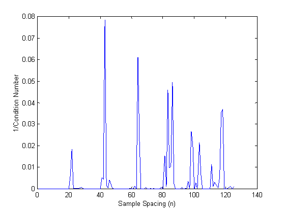
Figure
1: Inverse of the condition number of
the N-equation N-unknown matrices as a function of sample spacing (n) for 25
frequencies evenly-spaced from 0.1 to 1 MHz.
Large values indicate small condition numbers and ill-conditioned
matrices.
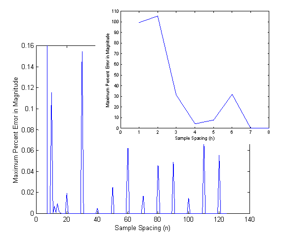
Figure
2a -- Error in the calculation of
magnitude using Gaussian Elimination for twenty-five frequencies evenly-spaced
from 0.1 to 1MHz where the inverse of the condition number is shown in Figure
1. Errors of less than 1% are obtained
for sample spacings greater than seven.
Errors for sample spacings less than seven (shown in inset to the right)
are 5-105% and are generally unusable.
This means that to compute magnitudes for twenty-five frequencies, the
last (7)(2)(25) time steps of the simulation would be required, or an
additional 350 time steps after convergence.
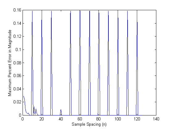
Figure
2b -- Error in the calculation of
magnitude using Singular Value Decomposition (SVD) for twenty-five frequencies
evenly-spaced from 0.1 to 1MHz . Errors
of less than 1% are obtained for all sample spacings. The magnitude and phase can be computed for
all twenty-five frequencies from the last 50 time steps of the simulation.
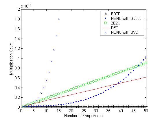
Figure
3: Computational requirements of the
FDTD algorithm and associated time-to-frequency domain conversions for the
parameter values indicated below Table 1.
This figure includes all FDTD simulation time steps necessary for each
method.
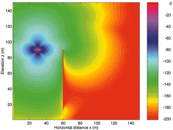
Figure
4: Horizontal magnetic field amplitudes
for a perfectly conducting slab (shown as the vertical line) illuminated by a
small loop (star-shaped element on upper left) at 2 MHz. This application seeks optimal receiver
location to the right of the slab to delineate slab location and size from a
source on the left. Values are expressed
in decibels relative to the maximum value.
The minimum has been clipped at –500 dB.
From [32].
Table
1: Computational Requirements for
Time-to-Frequency Conversion Methods
Table
2: Computational requirements for several different classes of
simulations. For all cases the FDTD
space is 100 x 100 x 100, and the
simulation is run for 2000 time steps.
Comparisons are made between simulations with one frequency (NF=1) and
twenty-five frequencies (NF=25). Values
shown for time-to-frequency domain methods do NOT include FDTD time steps.
Figure
1: Inverse of the condition number of
the N-equation N-unknown matrices as a function of sample spacing (n) for 25
frequencies evenly-spaced from 0.1 to 1 MHz.
Large values indicate small condition numbers and ill-conditioned
matrices.
Figure
2a -- Error in the calculation of
magnitude using Gaussian Elimination for twenty-five frequencies evenly-spaced
from 0.1 to 1MHz where the inverse of the condition number is shown in Figure
1. Errors of less than 1% are obtained
for sample spacings greater than seven.
Errors for sample spacings less than seven (shown in inset to the right)
are 5-105% and are generally unusable.
This means that to compute magnitudes for twenty-five frequencies, the
last (7)(2)(25) time steps of the simulation would be required, or an
additional 350 time steps after convergence.
Figure
2b -- Error in the calculation of
magnitude using Singular Value Decomposition (SVD) for twenty-five frequencies
evenly-spaced from 0.1 to 1MHz . Errors
of less than 1% are obtained for all sample spacings. The magnitude and phase can be computed for
all twenty-five frequencies from the last 50 time steps of the simulation.
Figure
3: Computational requirements of the
FDTD algorithm and associated time-to-frequency domain conversions for the
parameter values indicated below Table 1.
This figure includes all FDTD simulation time steps necessary for each
method.
Figure
6: Horizontal magnetic field amplitudes
for model B at 2 MHz expressed in
decibels relative to the maximum value.
The minimum has been clipped at –500 dB.
Figure
4: Horizontal magnetic field amplitudes
for a perfectly conducting slab (shown as the vertical line) illuminated by a
small loop (star-shaped element on upper left) at 2 MHz. This application seeks optimal receiver location
to the right of the slab to delineate slab location and size from a source on
the left. Values are expressed in
decibels relative to the maximum value.
The minimum has been clipped at –500 dB.
From [32].
Table 1:
Computational Requirements for Time-to-Frequency Conversion Methods
|
|
Multiplications
or Divisions |
Number
of FDTD simulations |
Storage
Locations |
|
FDTD
only |
9
NFDTDNxyz |
1 |
7
Nxyz |
|
DFT
** |
2
NFDTDNPxyz NPNF |
NF
(CW
FDTD) |
2NP NF NPxyz |
|
FFT ** (Radix
2: NFDTD
must be 2n) |
2
NFDTD log
2 (NFDTDNPxyzNP) |
1
(pulsed
FDTD) |
2NP NPxyz NFDTD |
|
2E2U
(storing
t1) |
4
NPNPxyz |
NF (CW FDTD) |
NPNPxyz |
|
2E2U (no
storage -- use last two time steps) |
4
NPNPxyz |
NF
(CW
FDTD) |
0 |
|
NENU |
9NDFDTDNxyz +12NPxyzNP(2NF)
3 |
1
(pulsed
FDTD) |
(2
NF)2 NPxyz NP |
Values
used in Figure 1
NFDTD
= # of FDTD time steps =
2000
Nxyz =
# of FDTD cells =
100 x 100 x 100
NF =
# of frequencies of interest =10
NP = # of parameters of interest = 6 (all E and all H)
NPxyz = # of FDTD cells of interest = 100 x 100 x 100
**
Complex multiplications in DFT and FFT are given the weight of approximately 2
real multiplications
Table
2: Computational requirements for several different classes of simulations. For all cases the FDTD space is 100 x 100 x 100, and the simulation is run for
2000 time steps. Comparisons are made
between simulations with one frequency (NF=1) and twenty-five frequencies
(NF=25). Values shown for
time-to-frequency domain methods do NOT include FDTD time steps.
|
Multiplications
Required |
Impedance
NP
= 5 NPxyz
= 1 |
Radiation
Pattern NP=4x6 NPxyz
= 90x90 |
Field
Distribution NP=3 NPxyz
= 100x100x100 |
|||
|
NF
=1 |
NF=
25 |
NF
= 1 |
NF=25 |
NF=1 |
NF=25 |
|
|
FDTD
only |
1.8
x 1010 |
1.8
x 1010 |
1.8
x 1010 |
1.8
x 1010 |
1.8
x 1010 |
1.8
x 1010 |
|
DFT * |
2.0
x 104 |
5.0
x 105 |
7.8
x 108 |
1.9
x 1010 |
1.2
x 1010 |
3.0
x 1011 |
|
2E2U
** |
20 |
500 |
7.8
x 105 |
1.9
x 107 |
1.2
x 105 |
3.0
x 108 |
|
NENU
(Gaussian Elimination) *** |
20 |
2.0
x 105 |
1.8
x 107 |
8.1
x 109 |
8.0
x 106 |
1.2
x 1011 |
|
NENU
(SVD) *** |
880 |
1.4
x 107 |
5.2
x 107 |
5.3
x 1011 |
5.3
x 108 |
8.2
x 1012 |
* IF pulsed FDTD is used, no additional FDTD
time steps are required after convergence.
**
Requires a separate FDTD simulation for each frequency. This will negate efficiency for higher
numbers of frequencies.
***
Requires 2NF FDTD time steps past convergence