How
to use TDR:
(1) Start PCTDR on any one of the machines in the Anderson Lab.
You should find it in Start à Programs à PCTDR.
(2) Switch On the Power Supply. Make sure you are giving 12 volts DC power supply to the TDR.(Test it with Multimeter)
(3) Your monitor should show a window like this.
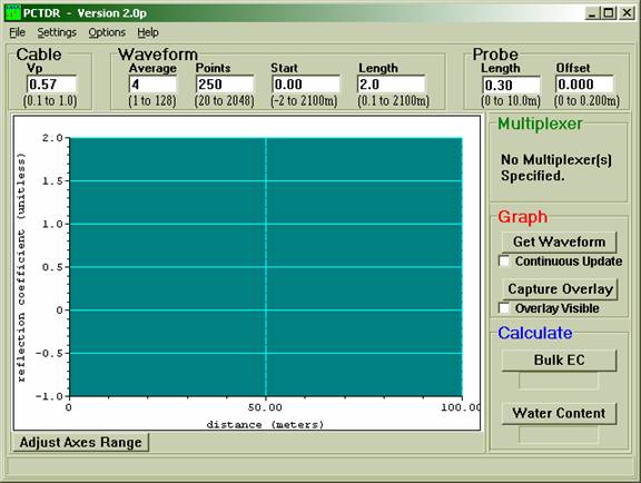
Vp is the ratio of the actual propagation velocity for a selected medium to the propagation velocity in a vacuum (3 *108 m-sec-1)
Specific Vp values for each coaxial cable are available from manufacturer data books. It is only necessary to know the Vp value if the TDR is being used for finding cable lengths or faults.
If you set the Vp as 1 it gives the apparent distance.
Apparent distance = Actual Distance * (Selected Vp / Actual Vp).
Say: If the actual length of the cable having a Vp of 0.78 is 5 meters and the selected Vp is 1.0, the apparent distance the end of the cable is 5*(1.0/0.78) = 6.41 meters)
Average sets the number of measurements averaged at a given distance from the TDR. A value of 4 is recommended.
Points – the number of points in the displayed or collected waveform. A value of 250 is recommended. A higher value can provide higher resolution
Start – to fix the start of the graph.
Length – to fix the span of the window of the TDR.
(4) Hook up a wire say RG58 coax.
Set Vp as 0.57, Average as 4, Points as 250, Start as 0, Length depending on the Physical wire u hooked up to the TDR.
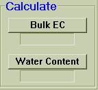
Following blocks are not required now. Just forget about them.


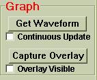
(5) After you hook up the wire. Click Get Waveform in the graph block.
Since the wire is not terminated with any Load. You will observe that the reflected Voltage is +1 as seen in the graph.
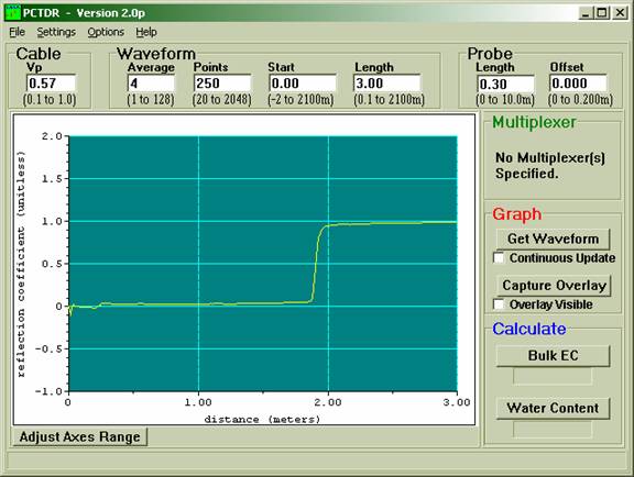
I hooked up a wire of 190 cms and there you can see that there is a jump in the waveform at 190 cm. This shows that cable is fine. If there is a fault in the cable then the jump will be somewhere below 190 cms. (Remember if you don’t put the Vp value as specified by the manufacturer then you wont get the jump at the exact point)
If you terminate the wire with a Short then you will see the following response.

If you terminate the wire with a matched Load then you will see the following response.

(6) Similarly Connect the Inductor, capacitor and resistor loads and see how the response is. (Hint: Inductor and capacitor act differently at t = 0 – and t > > 0).
(7) If you want to see how the waveform changes when u remove loads and put new ones to the end of the wire Check Continuous Update Field in the Graph block
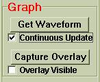
Similarly if you want to overlay graphs for all the loads make sure that Overlay Visible is checked in the Graph Block.
Saving data in TDR to plot Graphs in
Matlab:
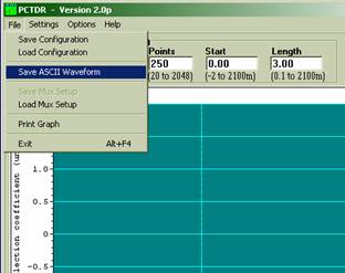
In the File Menu of the TDR Window, you have an option Save ASCII Waveform. Just click that and save the raw data from the TDR.
How to plot TDR plots using Data from the
TDR in Matlab:
(1) Open the file tdrplots.m
(2) Replace the file name ‘wire.dat’ with your ‘filename.dat’.
(3) Replace the word ‘wire’ with your ‘filename’ wherever you find it in the program.
The program gives you 2 plots (1) Reflected Voltage.
(2) Impedance Measurement.
v Reflected Voltage Graph is what you see in the TDR Reflection Coefficient graph. (Its actually reflected Voltage rather than Reflection Coefficient)
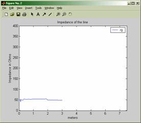
v From the Impedance Measurement plot, Zoom In the flat part in the graph and take the average that will give you the Impedance of the line as shown below.
(Here 50 indicates the Z0 of the cable attached)
(For better understanding of
how the TDR works U can check out the TDR
manual from ECE Stores)